4.4. Comparison of ring removal methods on challenging sinograms
Ring artifact is the most pervasive type of artifacts in tomographic imaging. Numerous approaches for removing this
artifact have been published over the years. In [R19], the author proposed many algorithms and a combination
of them (algorithm 6, 5, 4, and 3) to remove most types of ring artifacts. This combined method,
called algo-6543 for short, is easy-to-use and very effective. It has been implemented in Python, Matlab,
and available in several tomographic Python packages. To know more about causes of ring artifacts, types of ring
artifacts, and details of removal algorithms out of the original paper; users can check out the documentation page
here. This section demonstrates the performance of the
algo-6543 method
and sorting-based methods
in comparison with other methods on challenging sinograms. These data are available here
and free to use. They are very useful for testing ring removal methods.
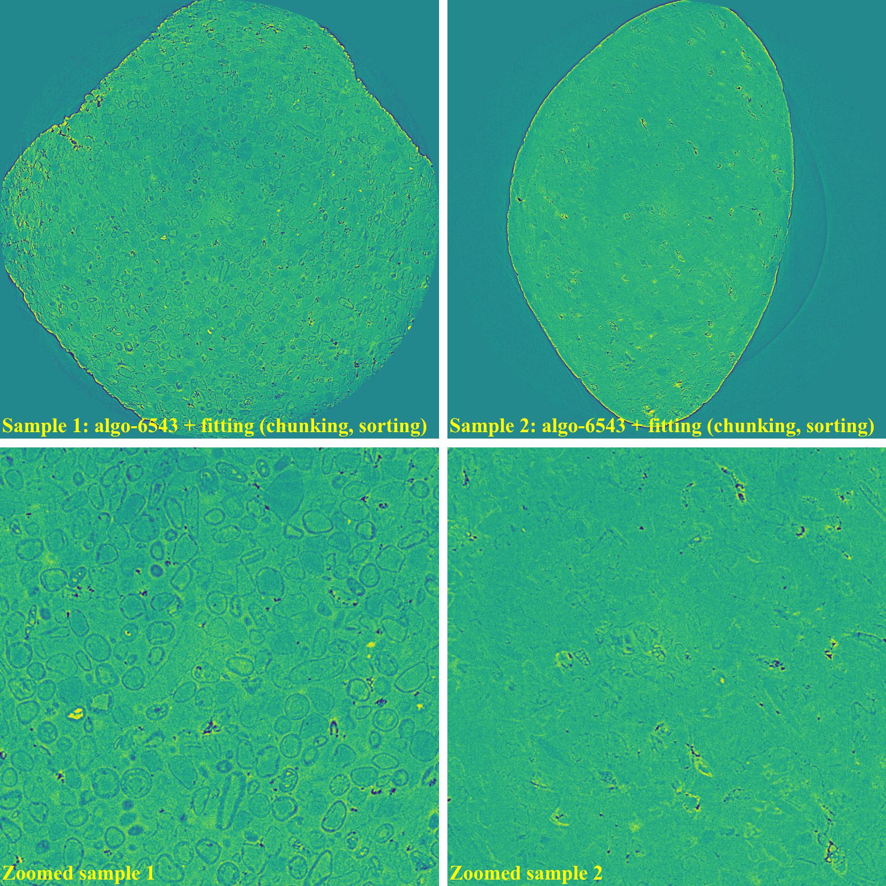
4.4.1. Same sample-type and slice but different in shape
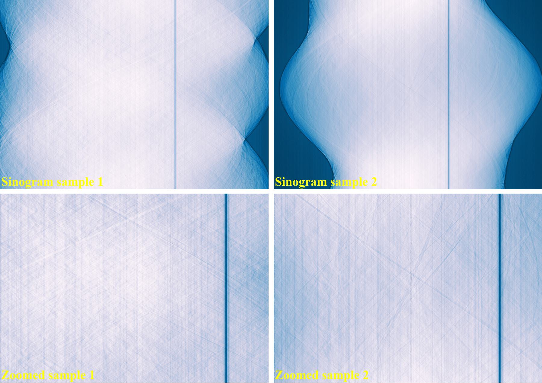
The following images show sinograms and reconstructed images of two limestone rocks with different shapes before and
after ring removal methods are applied.
Sinograms at the same detector-row:
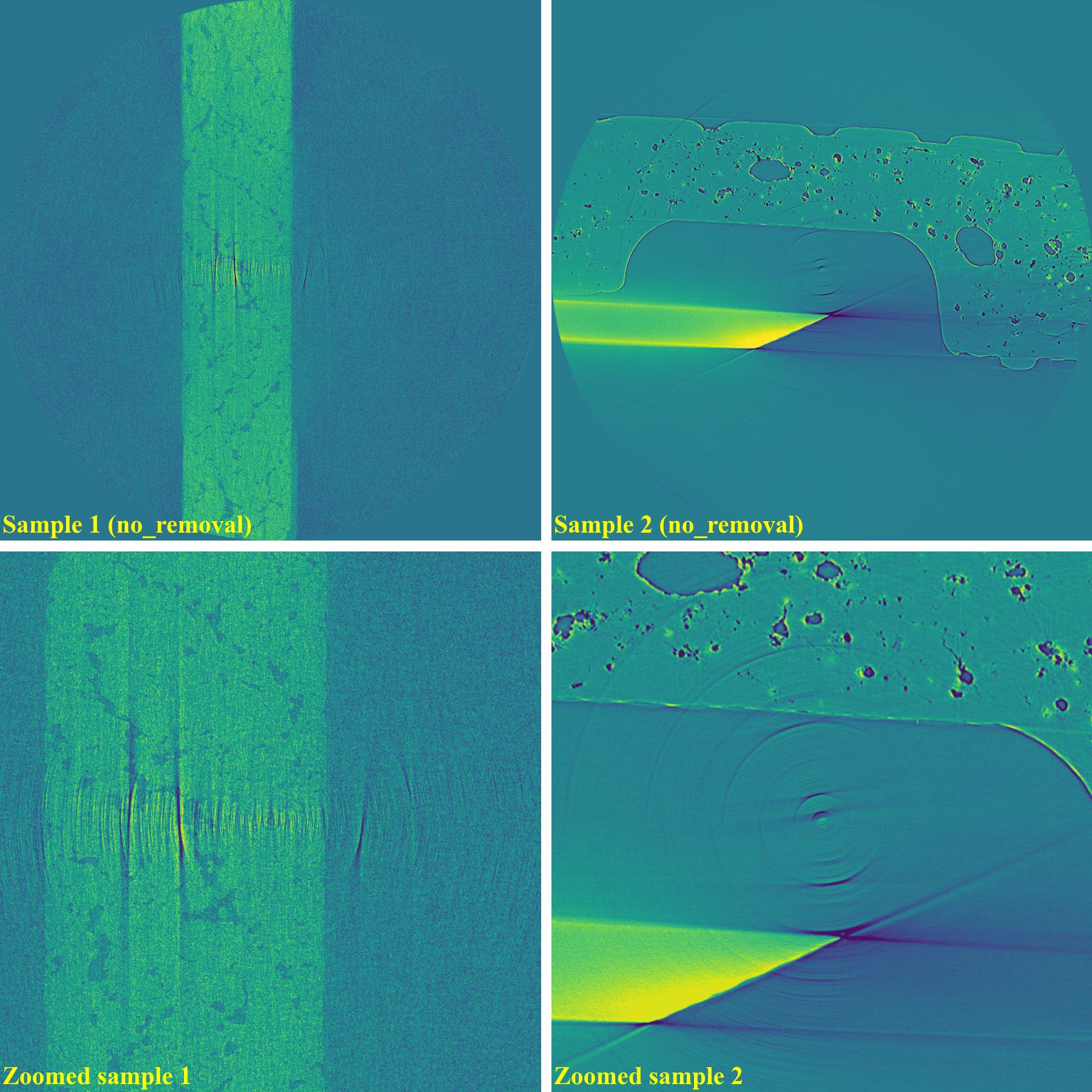
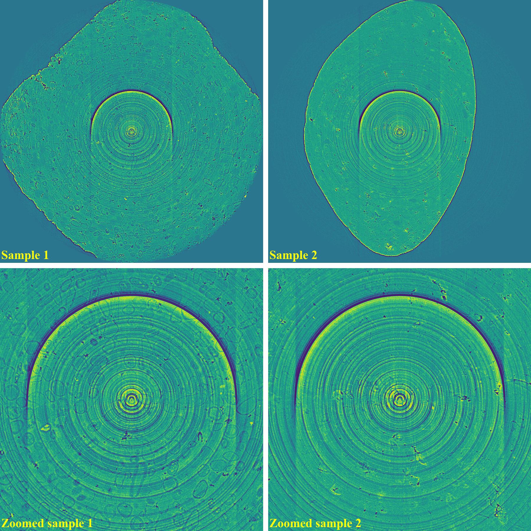
Reconstructed images without using a ring removal method:
As demonstrated, using the algo-6543 method gives the best results with least side-effect artifacts.
For other methods, it’s impossible to use the same parameters for different samples or slices.
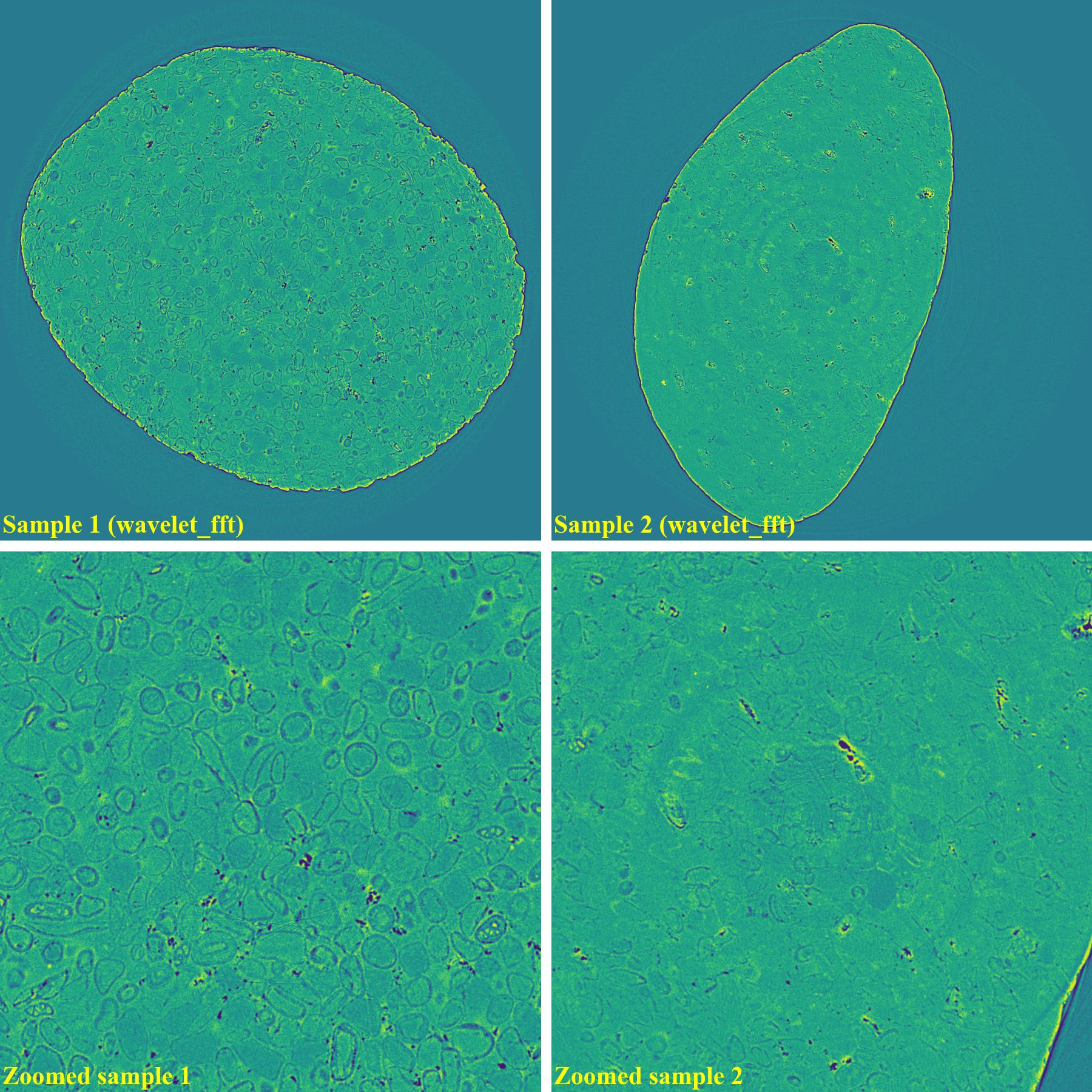
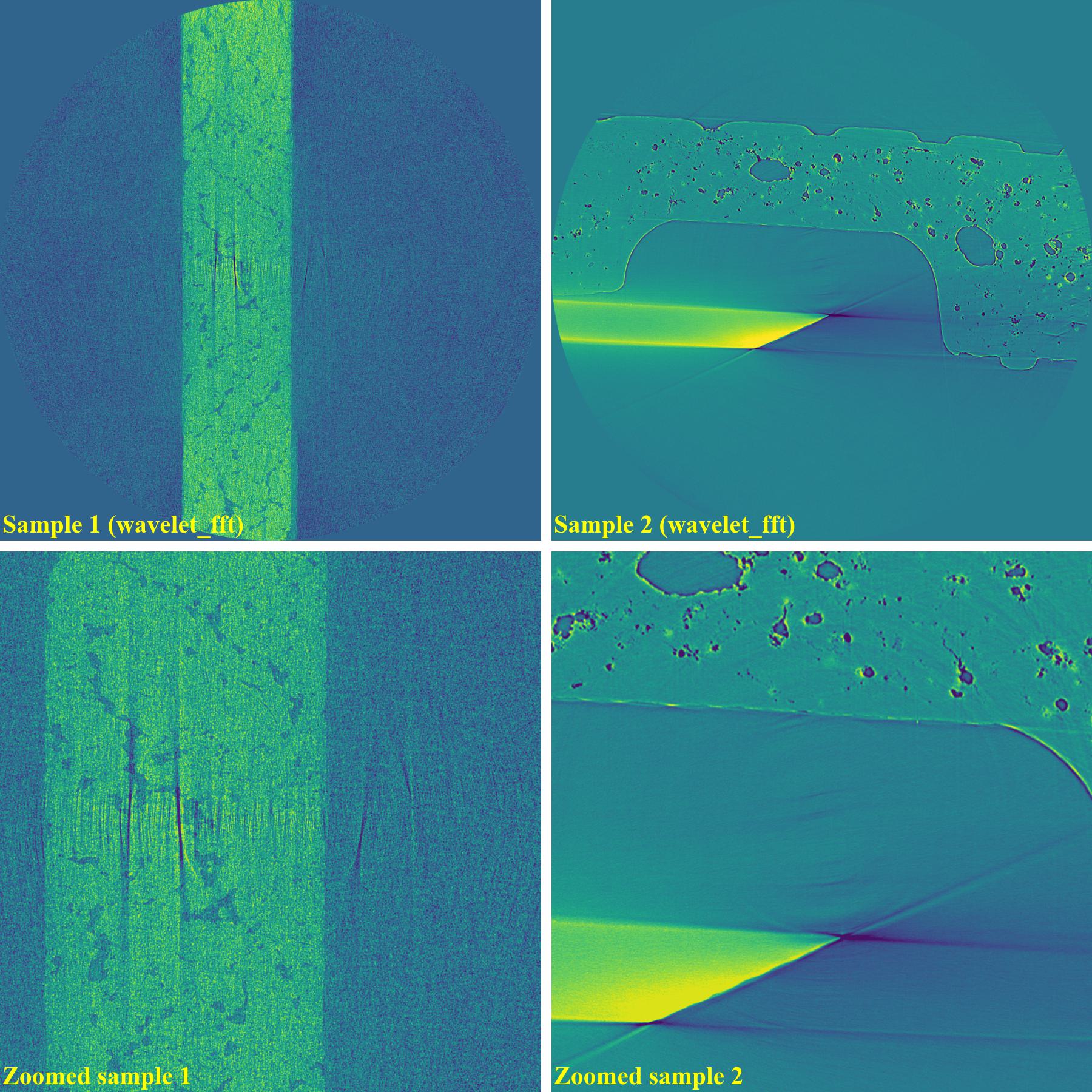
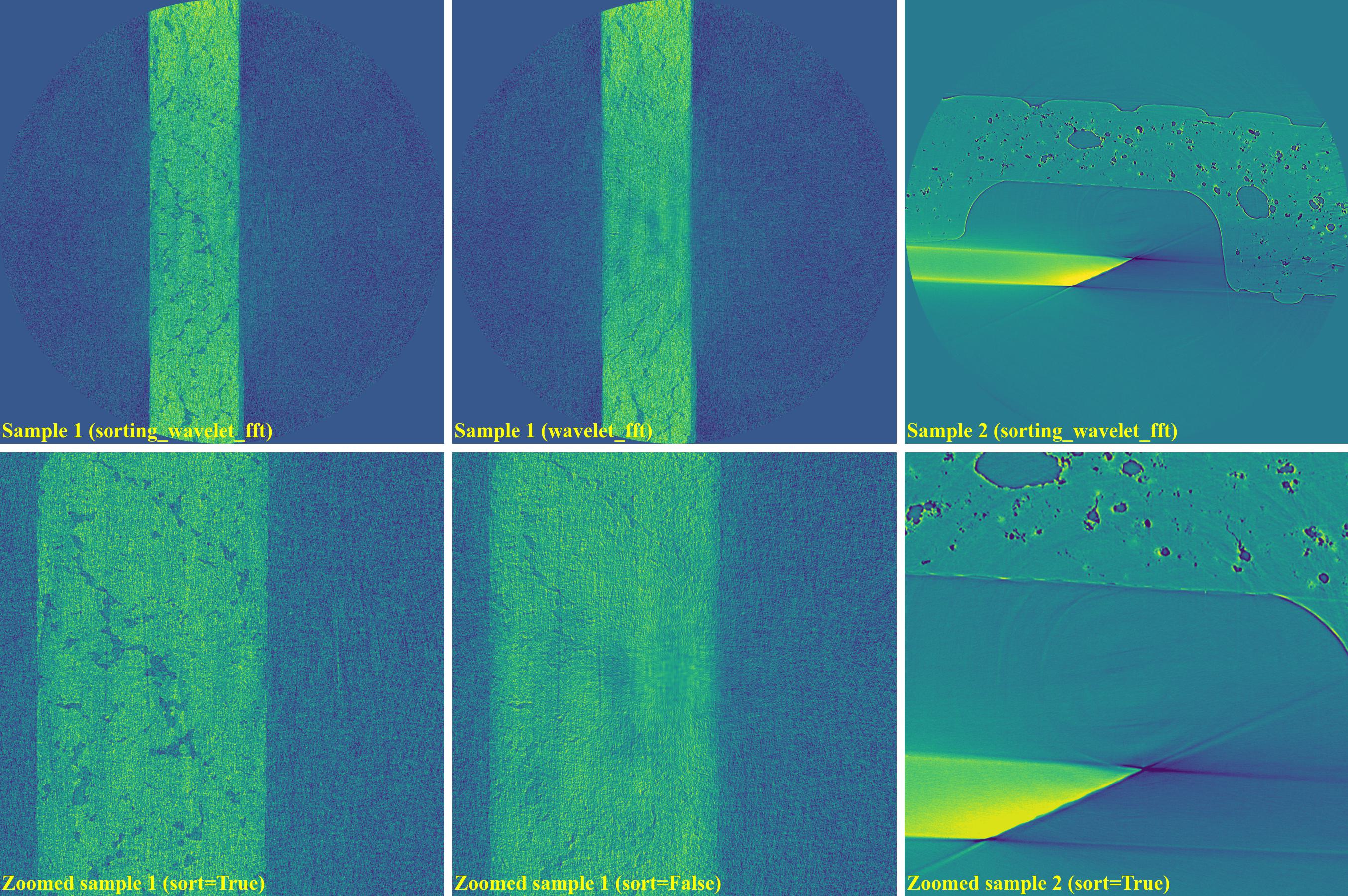
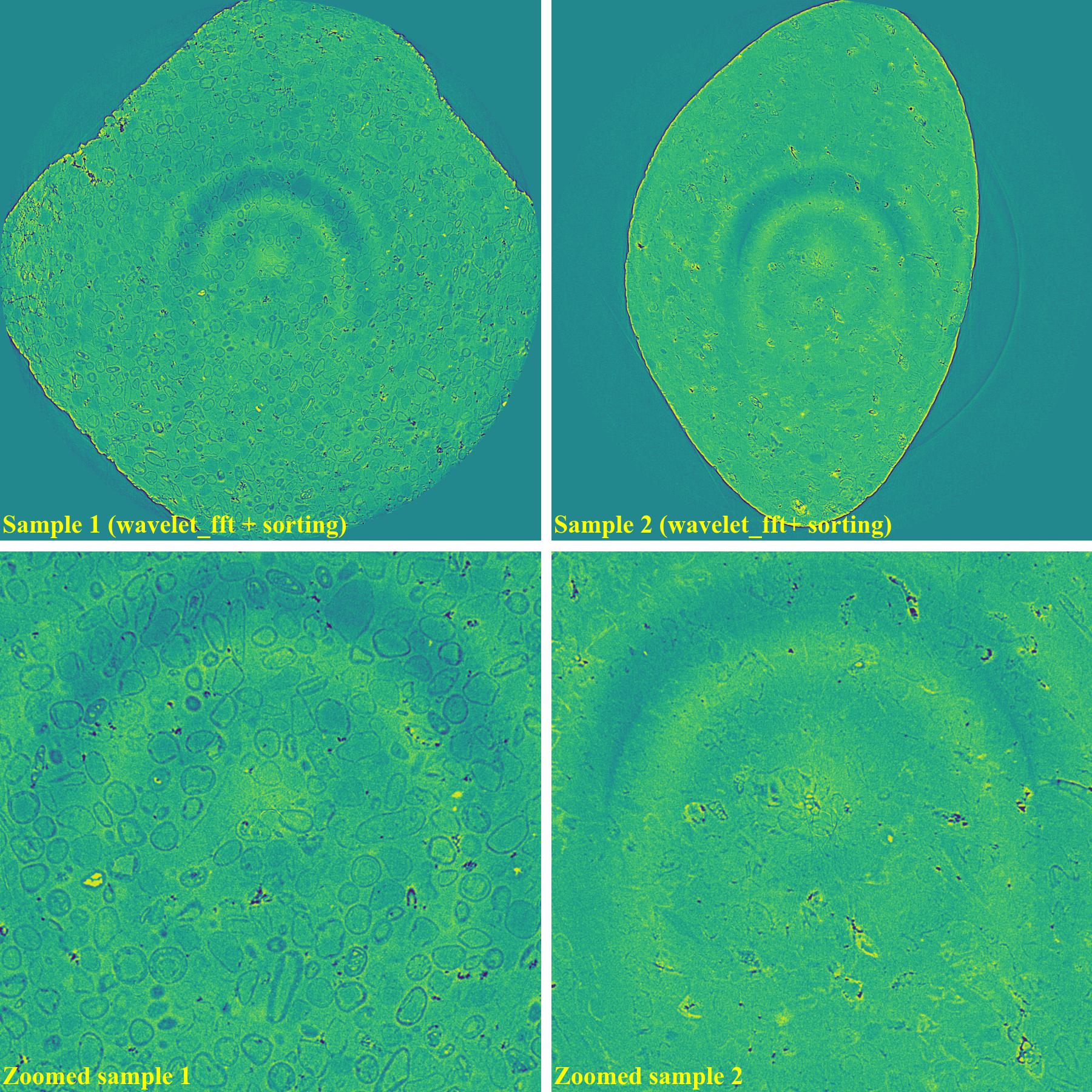
As can be seen, the original wavelet-fft-based method can’t remove partial rings effectively.
In Algotom, this method is improved by combining with the sorting method, which is the key part
of algorithm 3 in [R19]. This helps to avoid void-center artifacts when strong parameters
of the wavelet-fft-based method are used as demonstrated below
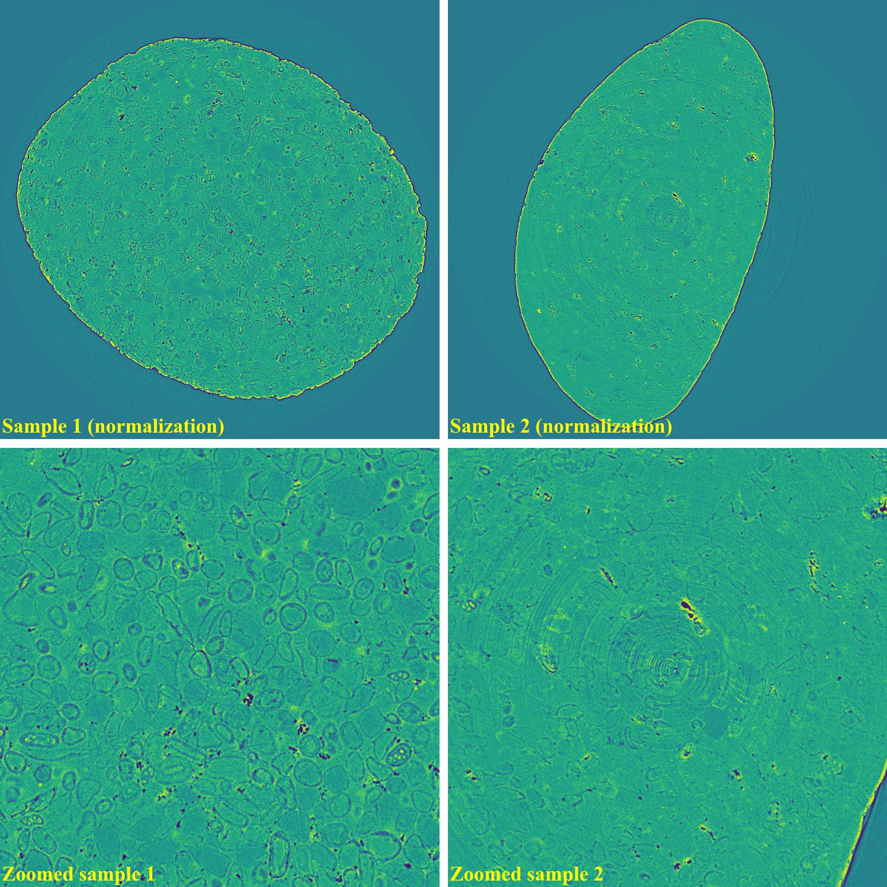
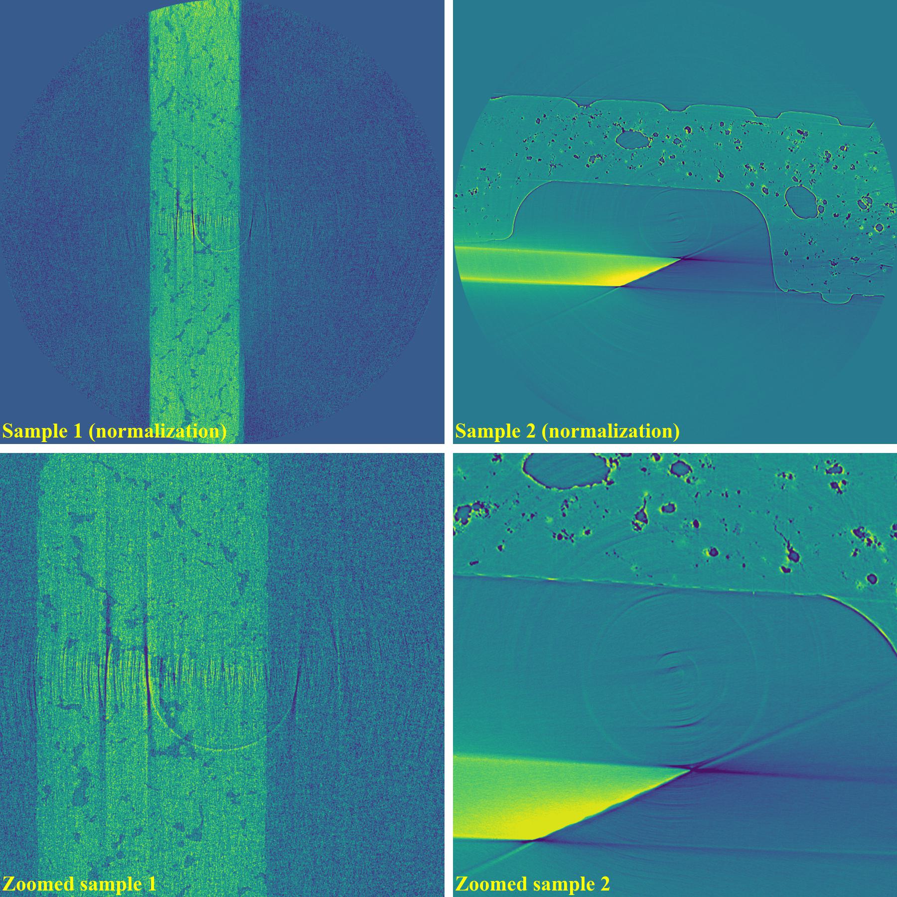
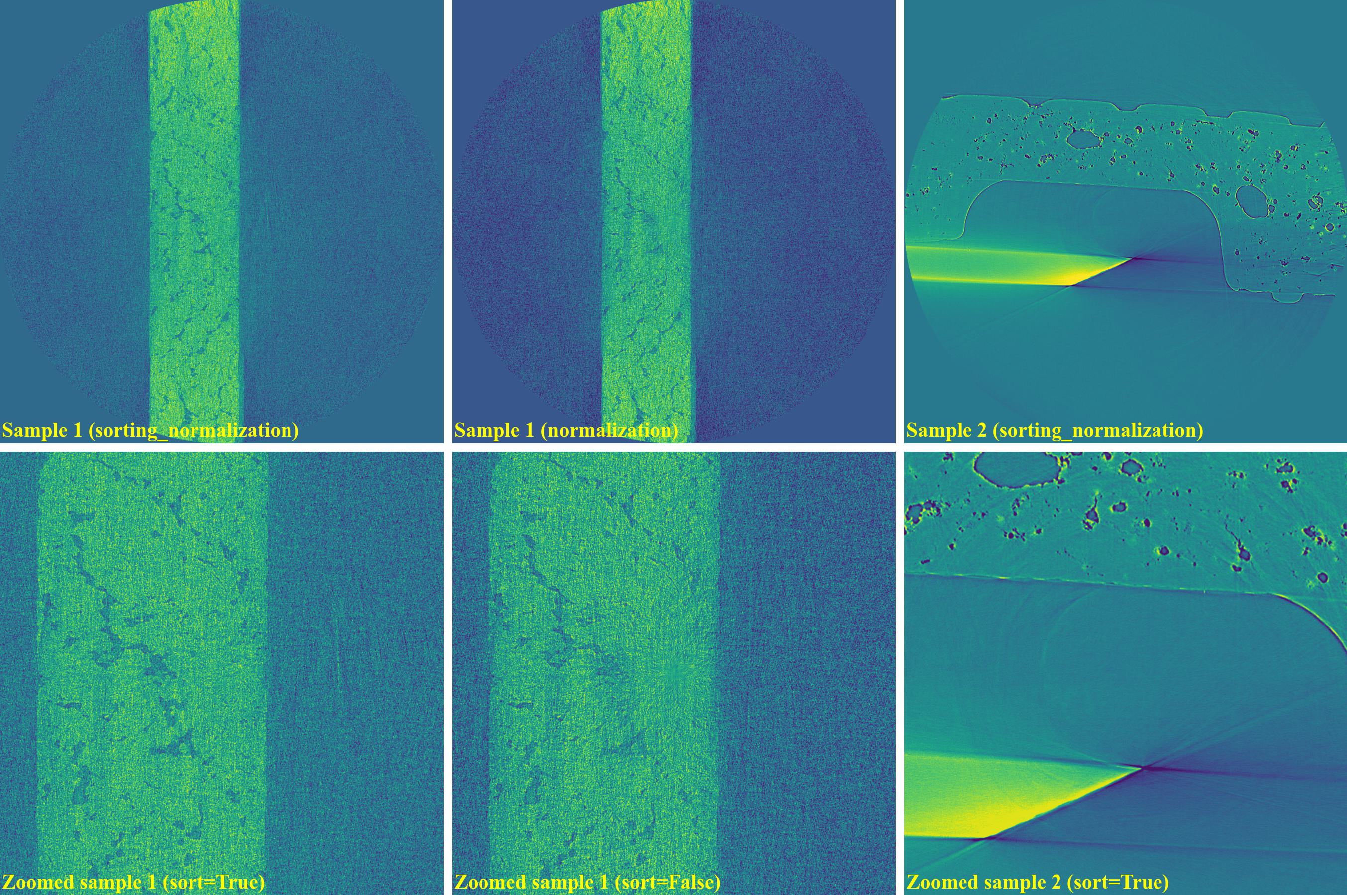
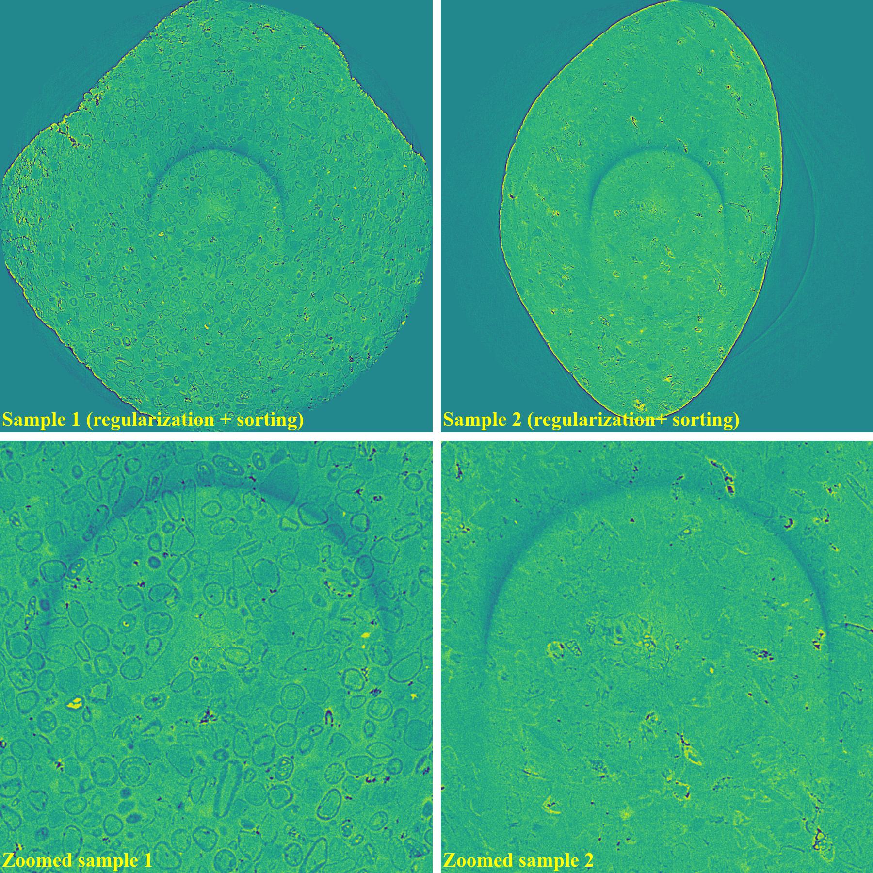
As shown above, the normalization-based method is not suitable for removing partial rings. However
it can be improved by dividing a sinogram into many chunks of rows and combining with the sorting
method.
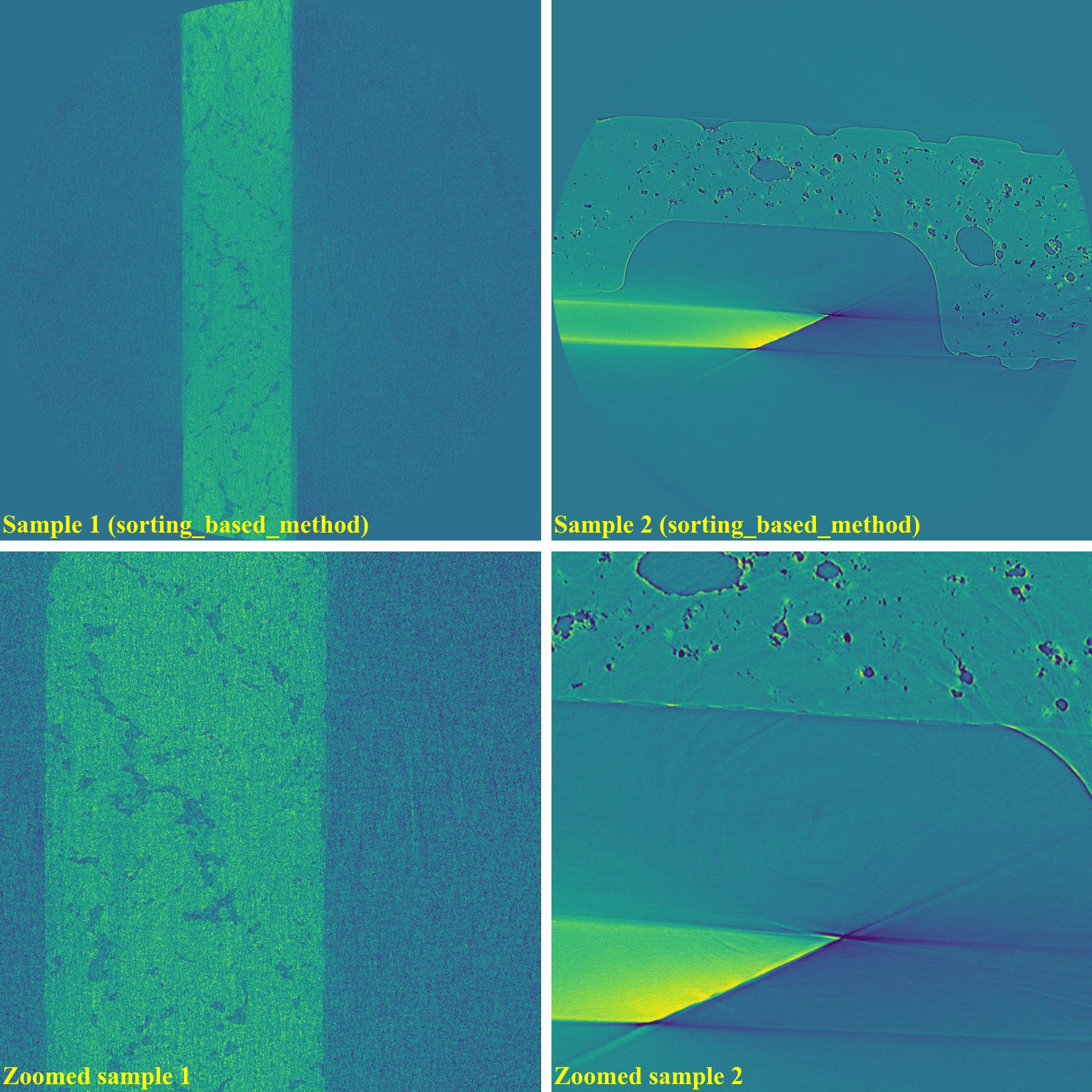
The above sub-section is to demonstrate the effectiveness of the sorting-based method in removing partial ring
artifacts and improving other methods in avoiding void-center artifacts. Results of using the fft-based method and
regularization-based method are not demonstrated here because their performance is similar to the wavelet-fft-based
method and the normalization-based method.
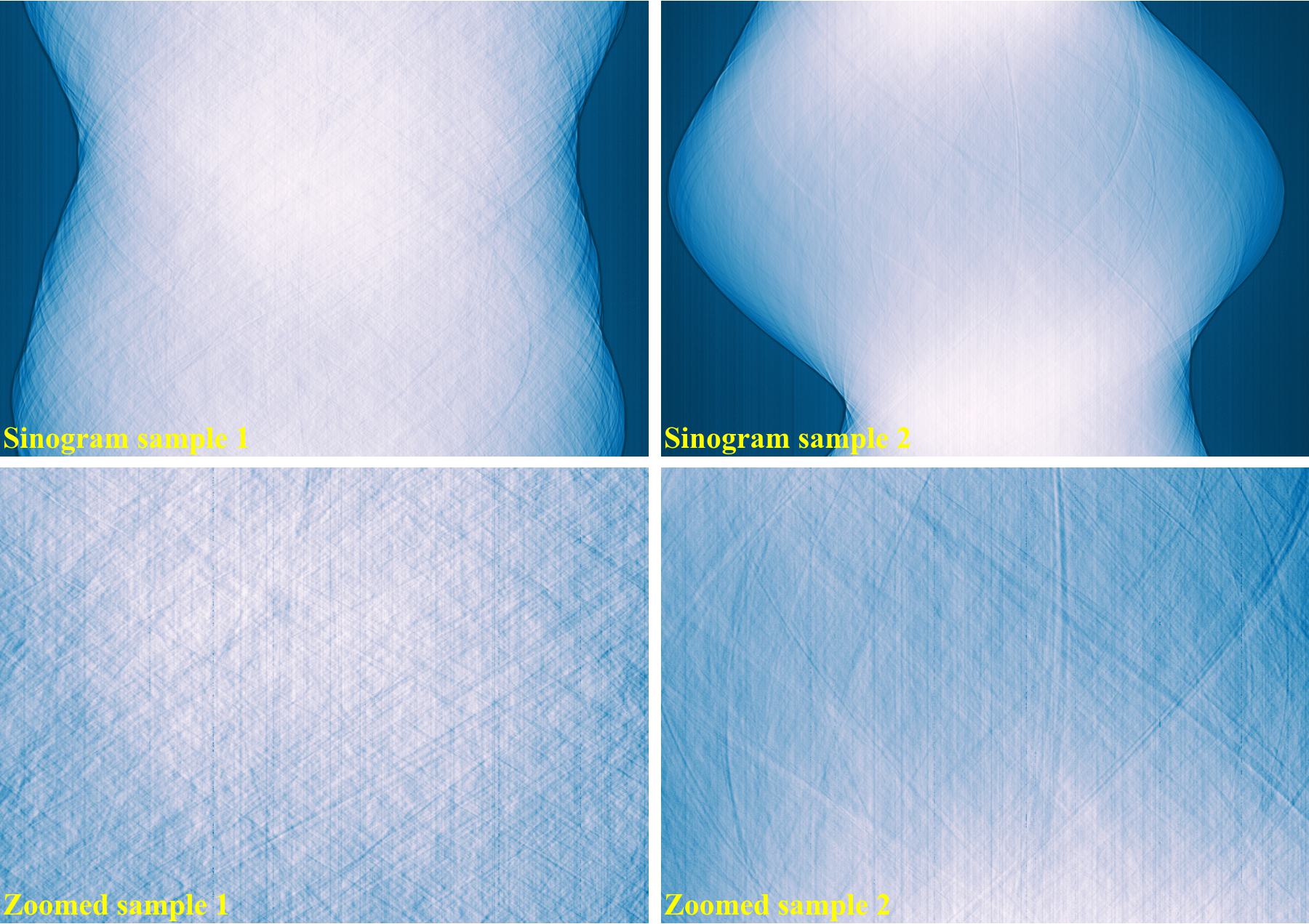
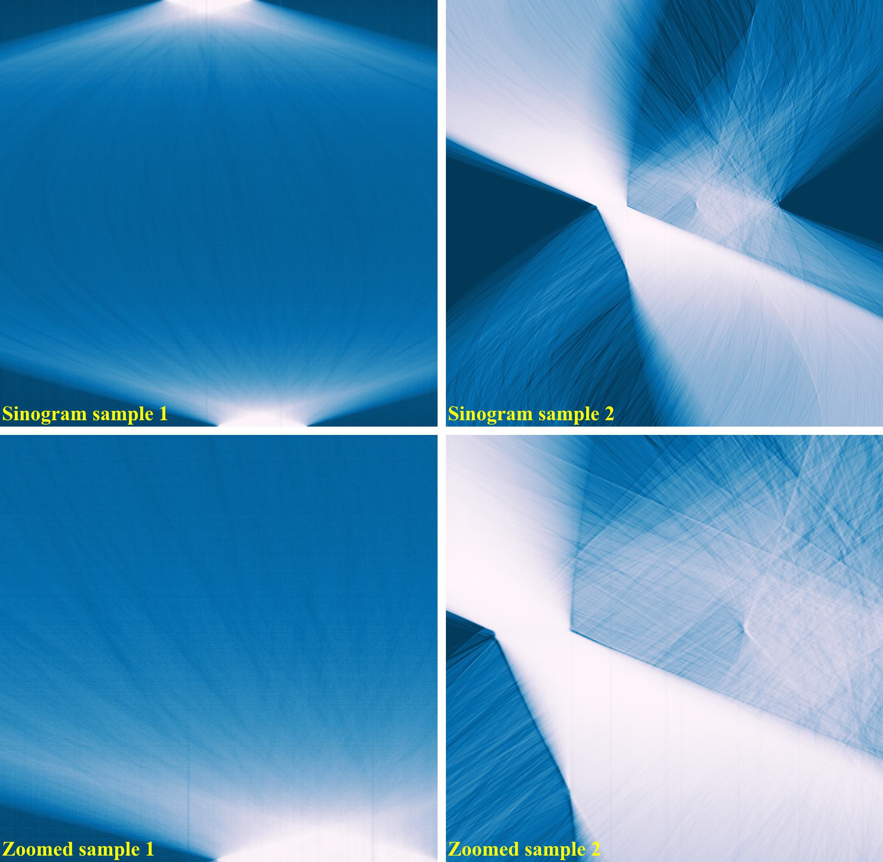
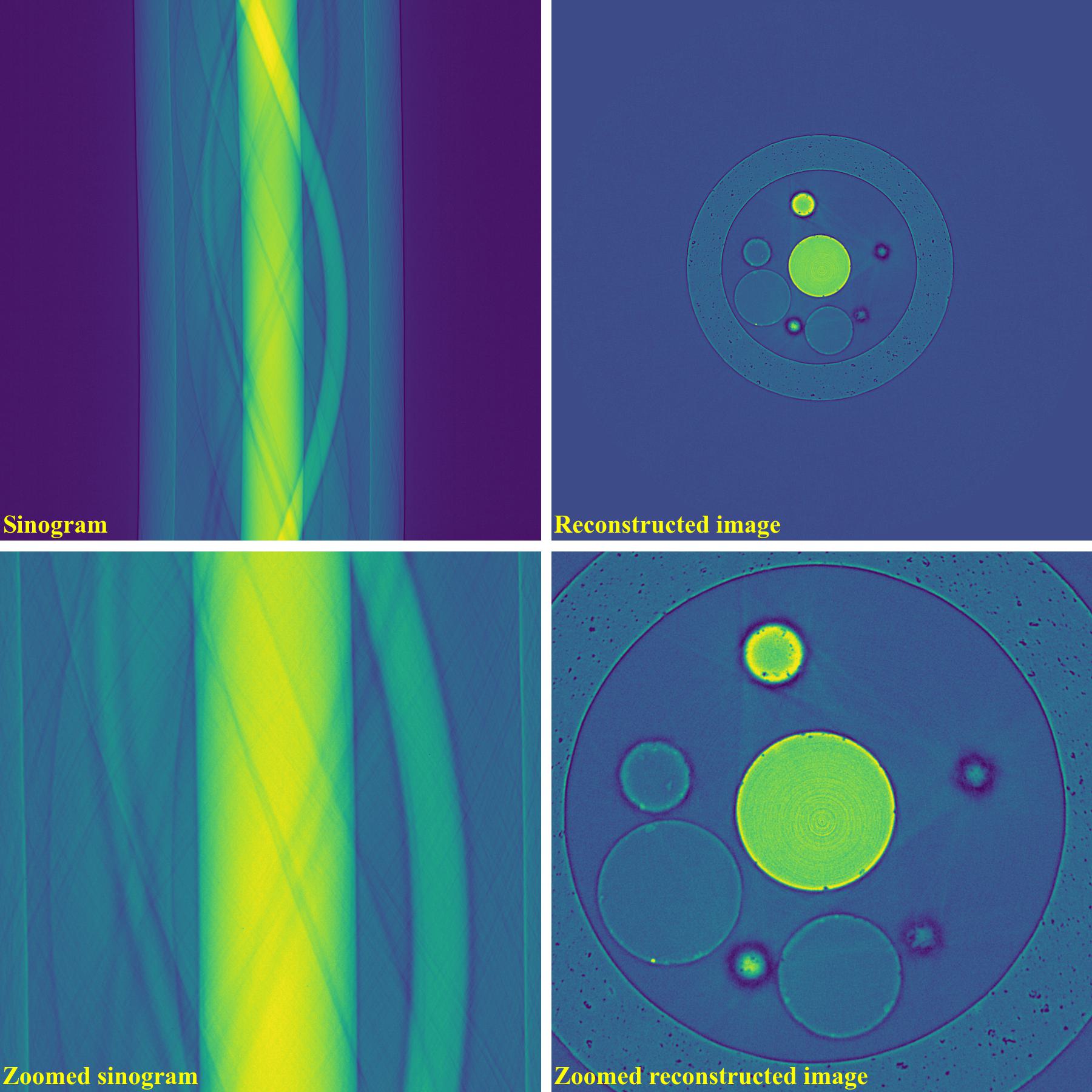
The following images show sinograms and reconstructed images of two limestone rocks with
different shapes having all types of stripe/ring artifacts
in one slice.
Sinograms:
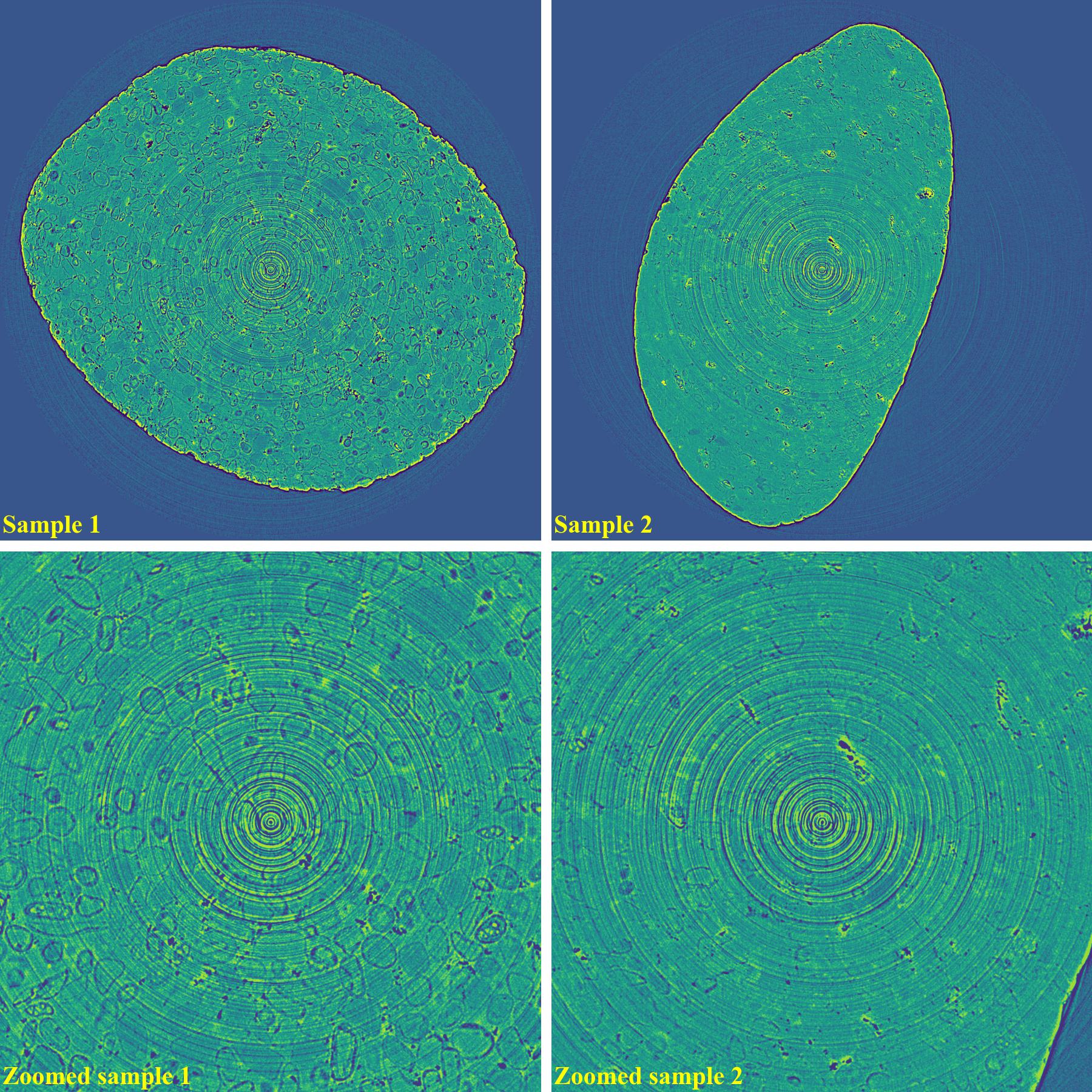
Reconstructed images without using a ring removal method:
As can be seen, there are still low-contrast ring artifacts which are difficult to detect and remove. These
low-contrast rings are caused by the halo effect
around blob areas on a scintillator. There is a strong removal method
proposed in [R19] and its improvement can help to deal with such ring artifacts as below.
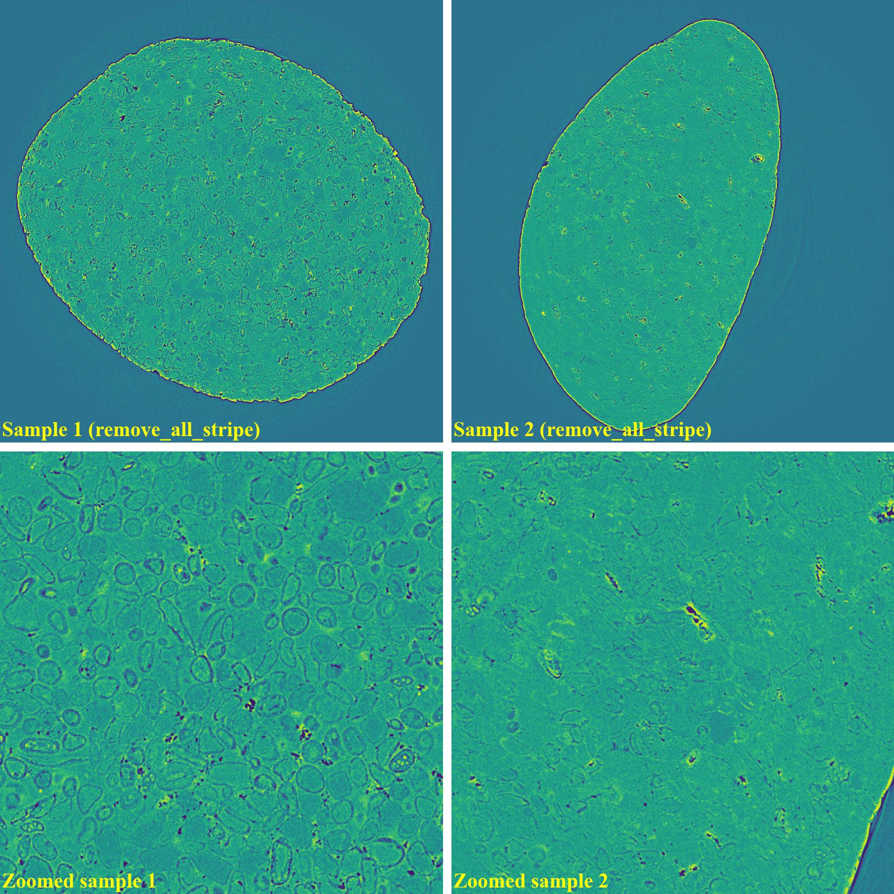
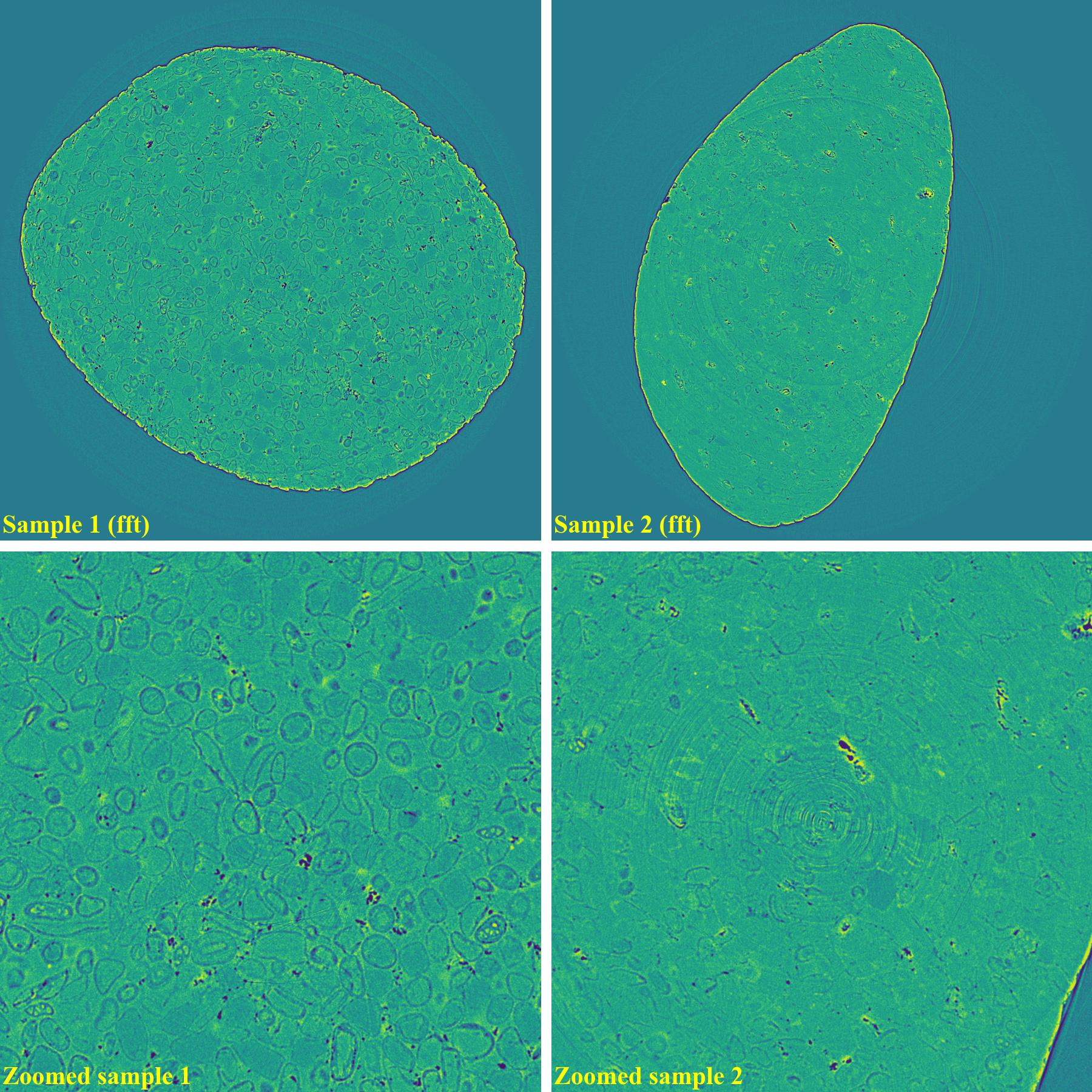
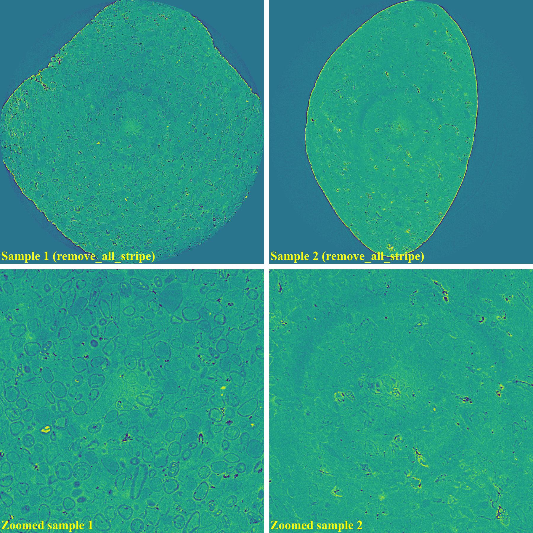
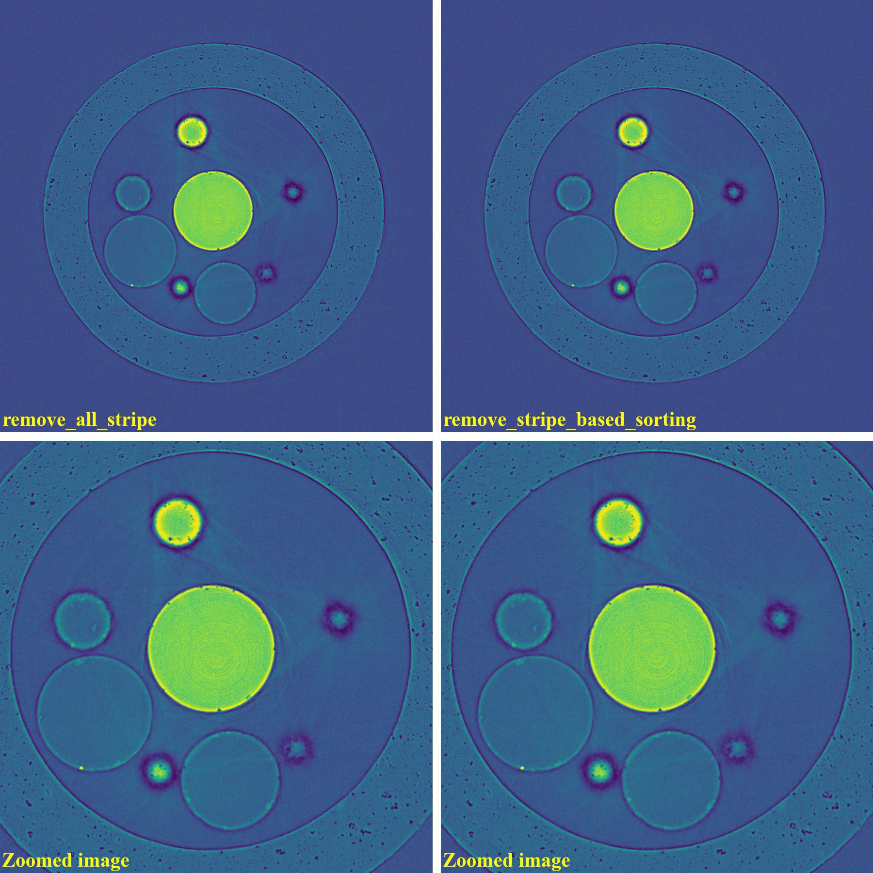
For samples containing round-shape objects (tubes, spheres), they can produce sinograms having valid stripes. This
is a problem for fft-based methods or normalization-based methods, but not for sorting-based methods.
Results of using the combined method and the sorting-based method as below. Note that the remaining ring artifacts
are insignificant. Although visible, they have nearly the same SNR (signal-to-noise ratio) as nearby background.
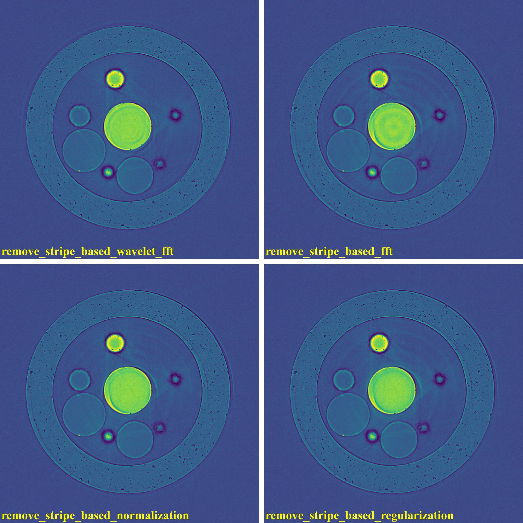
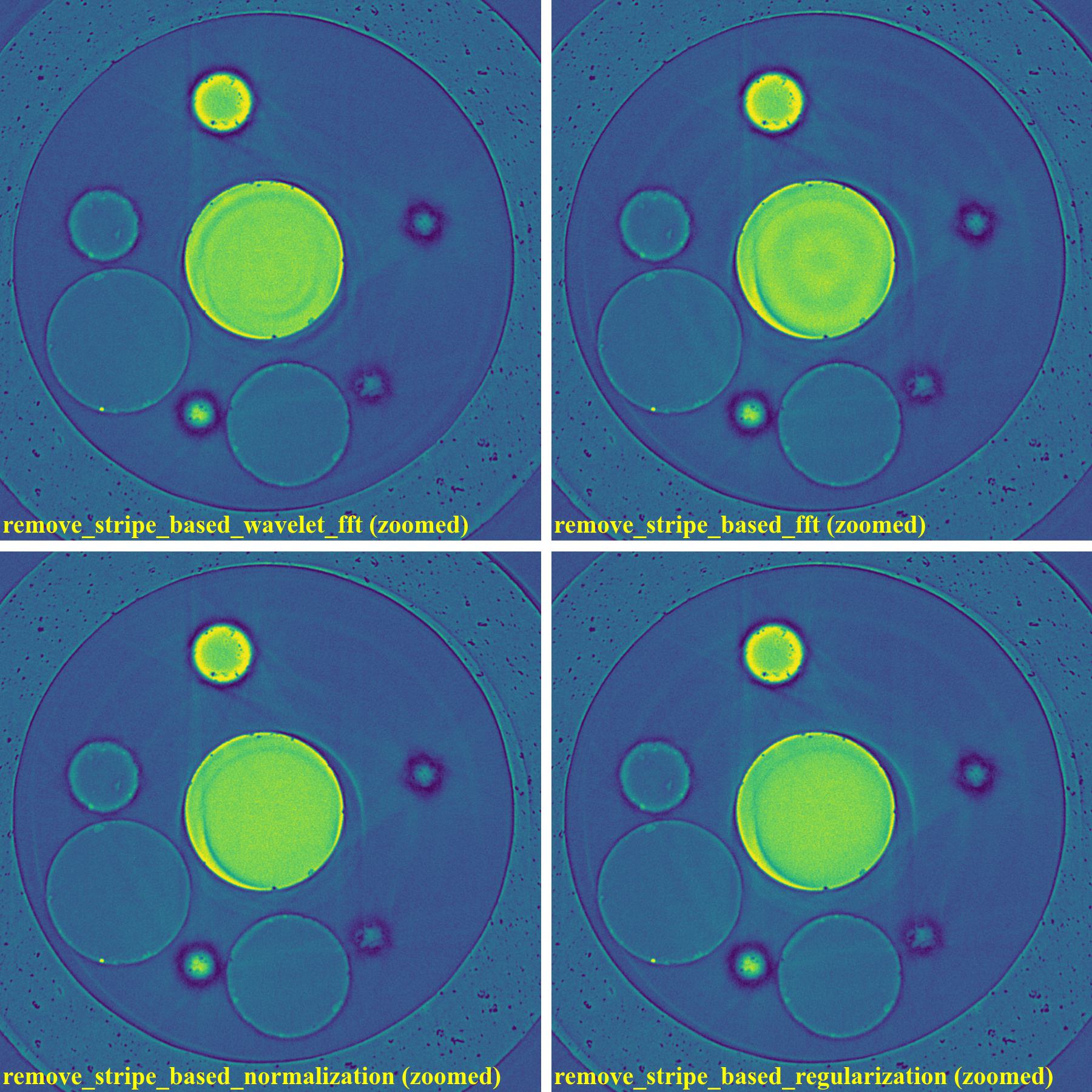
Results of using other methods are shown below. Although reduced strength, they still produce lots of
side-effect artifacts for such a pretty clean sinogram.
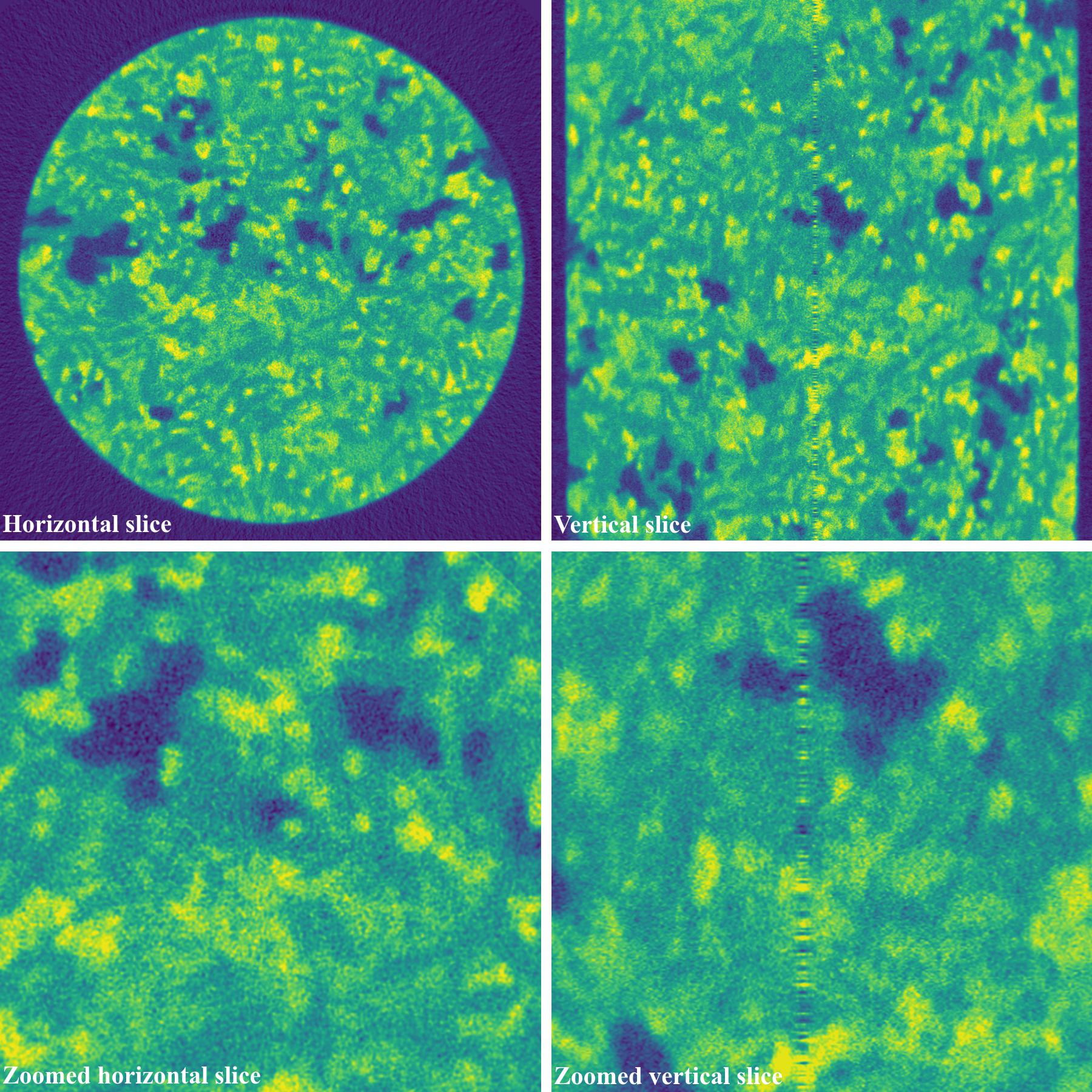
Post-processing ring-removal methods are often
used for cone-beam tomography because reconstruction can’t be done sinogram-by-sinogram. However, they can cause
void-center artifacts, which may not be visible in horizontal slices but clearly visible along vertical
slices. More than that, these methods can’t remove side effects of unresponsive-stripe artifacts
and fluctuating-stripe artifacts which not only give rise to
ring artifacts but also streak artifacts in a reconstructed image.
Certainly, we can apply pre-processing ring-removal methods along the sinogram direction. The only downside is that
we have to store intermediate results for switching between the projection space and the sinogram space.
It is common that commercial tomography systems output flat-field-corrected projection-images as 16-bit tif format (grayscale
in the range of 0-65535). The following shows how to apply pre-processing methods along the sinogram direction
step-by-step:
First of all, we convert tiffs to hdf file-format for fast slicing 3D data.
importtimeitimportnumpyasnpimportalgotom.io.converterasconvimportalgotom.io.loadersaveraslosainput_base="E:/cone_beam/rawdata/tif_projections/"output_file="E:/tmp/projections.hdf"t0=timeit.default_timer()list_files=losa.find_file(input_base+"/*.tif*")depth=len(list_files)(height,width)=np.shape(losa.load_image(list_files[0]))conv.convert_tif_to_hdf(input_base,output_file,key_path='entry/data',crop=(0,0,0,0))t1=timeit.default_timer()print("Done!!!. Total time cost: {}".format(t1-t0))
Then load the converted data and apply pre-processing methods. Note about the change of data shape
in each step.
importtimeitimportmultiprocessingasmpimportnumpyasnpimportalgotom.io.loadersaveraslosaimportalgotom.prep.removalasremimportalgotom.prep.correctionascorrimportalgotom.util.utilityasutilinput_file="E:/tmp/projections.hdf"output_file="E:/tmp/tmp/projections_preprocessed.hdf"data=losa.load_hdf(input_file,key_path='entry/data')(depth,height,width)=data.shape# Note that the shape of output data is (height, depth, width)# for faster writing to hdf file.output=losa.open_hdf_stream(output_file,(height,depth,width),data_type="float32")t0=timeit.default_timer()# For parallel processingncore=mp.cpu_count()chunk_size=np.clip(ncore-1,1,height-1)last_chunk=height-chunk_size*(height//chunk_size)foriinnp.arange(0,height-last_chunk,chunk_size):sinograms=np.float32(data[:,i:i+chunk_size,:])sinograms=util.parallel_process_slices(sinograms,rem.remove_all_stripe,[3.0,51,21],ncore=ncore,prefer="processes",axis=1)# Apply beam hardening correction if need to# sinograms = util.parallel_process_slices(sinograms,# corr.beam_hardening_correction,# [40, 2.0, False],# ncore=ncore, prefer="processes",# axis=1)output[i:i+chunk_size]=np.moveaxis(sinograms,1,0)t1=timeit.default_timer()print("Done sinograms: {0}-{1}. Time {2}".format(i,i+chunk_size,t1-t0))iflast_chunk!=0:sinograms=np.float32(data[:,height-last_chunk:height,:])sinograms=util.parallel_process_slices(sinograms,rem.remove_all_stripe,[3.0,51,21],ncore=ncore,prefer="processes",axis=1)# Apply beam hardening correction if need to# sinograms = util.parallel_process_slices(sinograms,# corr.beam_hardening_correction,# [40, 2.0, False],# ncore=ncore, prefer="processes",# axis=1)output[height-last_chunk:height]=np.moveaxis(sinograms,1,0)t1=timeit.default_timer()print("Done sinograms: {0}-{1}. Time {2}".format(height-last_chunk,height-1,t1-t0))t1=timeit.default_timer()print("Done!!!. Total time cost: {}".format(t1-t0))
Processed sinograms in the hdf-file then can be converted to 16-bit tiff images (i.e. to be used by cone-beam
reconstruction software provided by tomography-system suppliers). Otherwise, Astra Toolbox
can be used for reconstruction without the need of this conversion step.
importtimeitimportmultiprocessingasmpimportnumpyasnpimportalgotom.io.loadersaveraslosainput_file="E:/tmp/projections_preprocessed.hdf"output_base="E:/tmp/tif_projections/"data=losa.load_hdf(input_file,key_path='entry/data')# Note that the shape of data has been changed after the previous step# where sinograms are arranged along 0-axis. Now we want to save the data# as projections which are arranged along 1-axis.(height,depth,width)=data.shapet0=timeit.default_timer()# For parallel writing tif-imagesncore=mp.cpu_count()chunk_size=np.clip(ncore-1,1,depth-1)last_chunk=depth-chunk_size*(depth//chunk_size)foriinnp.arange(0,depth-last_chunk,chunk_size):mat_stack=data[:,i:i+chunk_size,:]mat_stack=np.uint16(data[:,i:i+chunk_size,:])losa.save_image_multiple(output_base,mat_stack,axis=1,overwrite=True,ncore=ncore,prefer='processes',start_idx=i)iflast_chunk!=0:mat_stack=np.uint16(data[:,depth-last_chunk:depth,:])# Convert to 16-bit data for tif-formatlosa.save_image_multiple(output_base,mat_stack,axis=1,overwrite=True,ncore=ncore,prefer='processes',start_idx=depth-last_chunk)t1=timeit.default_timer()print("Done!!!. Total time cost: {}".format(t1-t0))
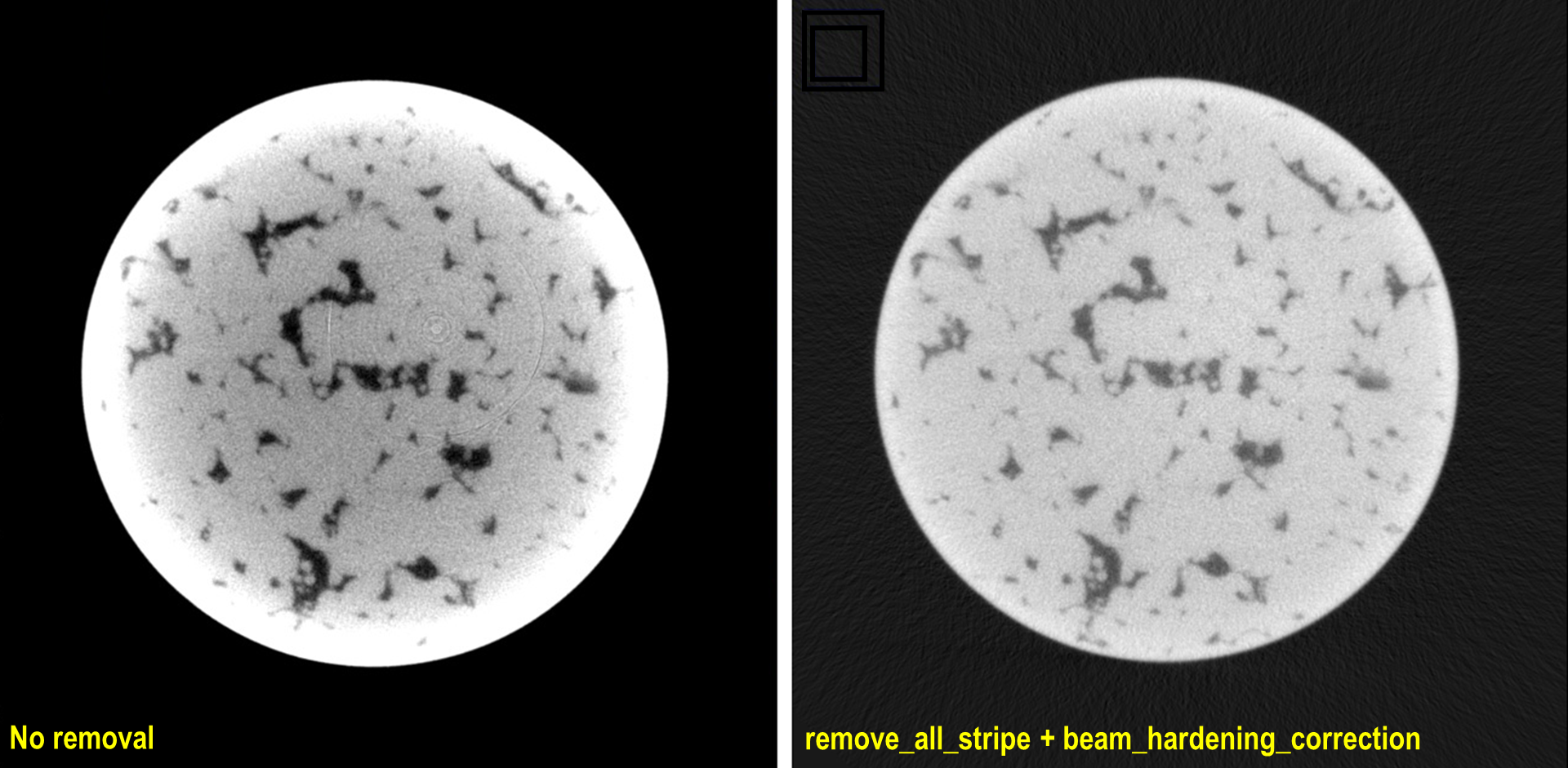
Fig. 4.4.1 Reconstructed images, before and after applied pre-processing methods, from projection-images acquired by
a commercial cone-beam system. Data provided by Dr Mohammed Azeem